Matic Jančič: Teaching portfolio - ACCESSING MARINE SPECIES OCCURENCES IN R WITH RGBIF

Summary

In this lab, you will be introduced to:

Global Biodiversity Information Facility (GBIF) database,
installing and loading R packages,
using R code to access the marine species occurrence data on GBIF server and download it,
data filtering and selecting to retain only information of interest,
simple visualization of spatial points.

What is Global Biodiversity Information Facility?

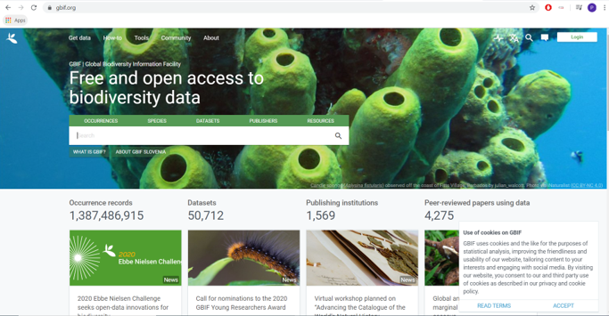
Global Biodiversity Information Facility (GBIF) is an international network and data infrastructure. It is funded by the world’s governments and aimed at providing anyone, anywhere, open access to data about all types of life on Earth.

At the time of writing this study materials, there were more than 2.2 billion records published in the GBIF database, in both marine and terrestrial realm on a global scale. The webpage itself is very practical in terms of navigation and search, but what is even better is that occurrence data can be easily accessed and downloaded through R either for a species or taxa of interest.

Task

Open the GBIF website and explore it for a couple of minutes.

Global Biodiversity Information Facility landing site some time ago

Data from GBIF can be downloaded manually and than imported to R. However, programmers are lazy, so biologists can be lazy as well, right? For that purpose, there is an R package called rgbif. It contains functions that enable us to contact GBIF server directly, communicate with it and get only the data that we are interested in. In R, we first need to install a package using install.packages() function with the name of the package in quotation marks within the parenthesis. This should automatically download and install the package. We also need to load the package each time that we start or restart R or RStudio. This is done with library() function with the name of package without quotation marks in the parenthesis. Each package commes with a document in which all important information are available, example for rgbif can be accessed here. More popular packages usually have informative “cheat sheets” as well (example later on).

Important

When installing R we “only” get access to some functionalities that are available. That is because there are really many available and individual user doesn’t need most of them. To add new functionalities, we need to install additional R packages from the internet (imagine R package as an add-on or extension of the base installation). Installation needs to be done only once, before the first use of the package!

However, installing the package does not make it available for use. Again, not all packages are needed all the time so we have to load the package each time we restart R or RStudio to be able to use it!

Task

Open an empty R script from the File dropdown menu by clicking New file \ R script. The script will have a name Untitled1 (or Untitled2, if a blank script was already open).

Save the script to the Desktop of your computer and name it Accessing marine species data with R.

Copy and paste below code to the R script, move cursor to the first row with code and click Run. Move cursor to each row that contains code and repeat.

install.packages("rgbif")
library(rgbif)

How to access species occurence data from GBIF?

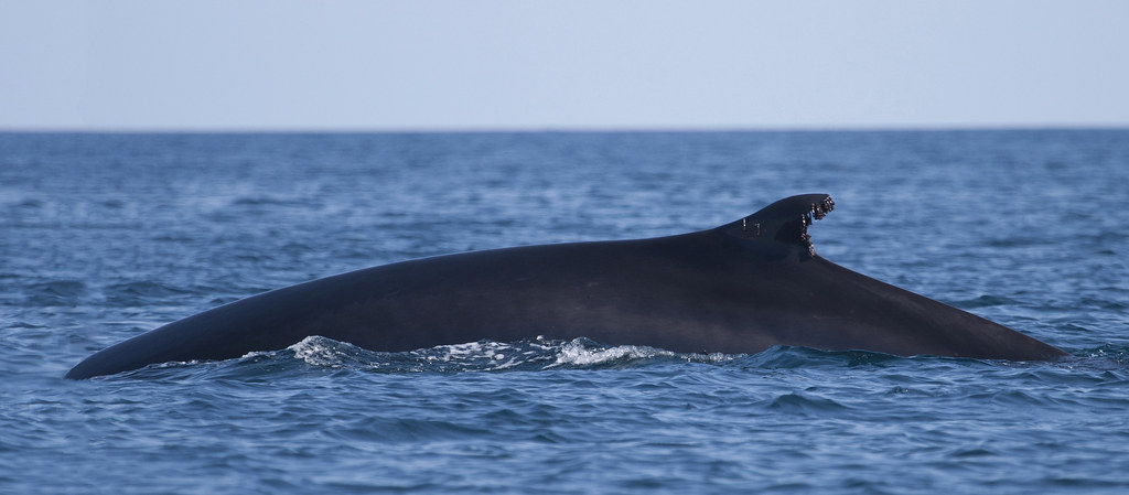
To access the occurrence data we will use occ_search() function, which will contact the GBIF server and download the data from the database. We will take the fin whale (Balaenoptera physalus) as an example.

Fin whale (photo credit: https://www.flickr.com/photos/slobirdr/29414853626)

We introduced functions yesterday and said that we give them some object to get a result. Apart from objects that we create, functions accept other input as well. This input can provided as different arguments of the functions, for example the occ_search() function has an argument called scientificName = NULL, set to NULL by default. If we want to use this function to search for fin whale occurences on GBIF server, we need to change it to scientificName = "Balaenoptera physalus". Note that the latin name is written within the quotation marks for R to treat it as a word. There are many arguments that we could use, to refine our search (i.e. hasCoordinate, country, continent, etc.), but we will not use at this point.

Tip

If you ever need to get information about any R function, type the question mark before its name (without parenthesis) and its documentation will open in the Help tab.

Below code will first open the documentation for occ_search() function and than store the results of it to physalus_gbif object, which should appear in your Global environment shortly after running the code.

Task

Copy and paste below code to the R script, move cursor to the row with the code and click Run. Explore the document that will open in the Help tab.

Run the second line of the code and check your working directory, if a new object was created. As we will all be contacting the GBIF server at the same time, it might take a while for all requests to be processed and finished.

?occ_search

physalus_gbif <- occ_search(scientificName = "Balaenoptera physalus")

Right of physalus_gbif object you can see what type of an R object it is: a list of 5 elements. If you click on the small blue icon left of the physalus_gbif, its content will be displayed below. You can see that we actually downloaded a lot of stuff. There are three lists called meta, hierarchy and media (far below), and a tibble or dataframe called data. Fifth element is not even listed as the first four have so much content that it was not printed in this display. We could explore all of this elements, but will look only at the data part, where coordinates and other information on the records are stored. In the display, you can see a dollar sign ($) in front of an element name. This is not coincidence, as it tells us, that we can access this part of the list by adding $data after its name. We will save the result of this operation to yet another object, that we will name physalus_data, which is a dataframe and which will be our dataset for further exploration.

Task

Copy and paste below code to the R script, move cursor to the row with code and click Run. Check your working directory if a new object was created.

physalus_data <- physalus_gbif$data

Questions:

Is physalus_data indeed a dataframe (or a tibble) as it was the $data element of physalus_gbif?
How do you know that and is there an R function with which you can check that out?
How many rows and columns does physalus_data dataframe has?
How do you know that and are there R functions with which you can check that out?

Do you have any questions?

There are 500 observations of fin whales in the table, which is not necessarily the actual number of occurences in the database. To prevent server (over)load the default is to download 500 occurrences. This is the case for fin whales as well, as there are 113772 occurrences in the GBIF database (check here). To change the number of downloaded occurrences, we would need to change the argument limit = to the desired value (however, note that 100,000 is the maximum limit set by package creators).

Task

Click on the physalus_data object, its content should get displayed where your R script is open. Explore the table and try to identify columns that can be useful for us (i.e. coordinates, year, etc).

Note that everything in R can be done in multiple ways. We will look at filtering (using a condition and retain a subset of observations - rows) and selecting (retaining only columns of interest) parts of our data using dplyr R package. The same could be achieved using only base R or advanced packages such as data.table. R package dplyr is very suitable for R beginners as it is very intuitive, but nevertheless very useful and powerful. Remember from above, we need to firs install the package and than load it, for its functions to be available.

Task

Copy and paste below code to the R script, move cursor to the row with code and click Run. Check your working directory if a new object was created.

install.packages("dplyr")
library(dplyr)

For selecting columns of a dataframe we use select() function which takes two arguments: the name of data object we want to select from and the name of column we want to select. With select()we can choose multiple columns. Of more than 100 columns that were downloaded, only some have meaningful values for us at this moment. We will retain several, such as the species name (species), coordinates and its error measurement (coordinateUncertaintyInMeters). For filtering by row values we use filter() function which also takes two arguments: the name of data object we want to select from and the expression based on which we want to filter. For example, we do not want fin whale observation with large cordinate uncertatinty, right? To retain only those with 5 km or less, we simply need to specify the name of the column coordinateUncertaintyInMeters and the filtering condition (< 5000). 5 km is not that bad considering the movement capabilities of fin whales, right? We will save results of selecting and filtering in physalus_data object, which will overwrite the original object.

physalus_data <- 
  select(physalus_data,
         species,
         decimalLatitude,
         decimalLongitude,
         coordinateUncertaintyInMeters,
         country) %>% 
  filter(coordinateUncertaintyInMeters < 5000)

Tip

The %>% operator is used to “chain” operations meaning that one operation follows the next in the specified order and with that our code is more compact, efficient and readable. Below code is therefore read as:

select columns from physalus_data object
and (without additional specification) filter this smaller dataframe acoording to given condition.

Warning

Functions select() and filter() are defined in multiple R packages. Depending on which package was loaded last by library(), R chooses which version of the function it will apply. If we do not get the expected result from the function or an unexpected error after running it, this is the likeliest cause.

Tip

We can avoid problems with commonly named functions by telling R a priori which function from which package we want to use. For example, select() or filter() from dplyr as follows:

dplyr::filter(),
dplyr::select().

How to simply map the occurences?

Now that we have downloaded and filtered the data, we can simply display them on a map. Again, many options in R are available. We will use leaflet package which provides an easy way for creating interactive maps. The function for starting a map is leaflet() and we need to specify which object we want to map, in our case this will be physalus_data. Next, we use addProviderTiles() to add a background to our map. We also need to select one of the available options, for example provider = "Esri.WorldImagery" we specify which type of background. You can explore other options for background here. You change the background by replacing "Esri.WorldImagery" with another name, i.e. "OpenTopoMap". Next we add our points with function addCircleMarkers(), within which we must specify names of columns in our data that represent longitude (lon) and latitude (lat).

Task

Copy and paste below code to the R script, move cursor to the row with code and click Run. Move cursor to each row that contains code and repeat. The code starting with leaflet(physalus_data) should run from the start to the end after one click on Run

install.packages("leaflet") 
library(leaflet)

leaflet(physalus_data) %>%
    addProviderTiles("Esri.WorldImagery") %>%
    addCircleMarkers(lng = ~ decimalLongitude,
                     lat = ~ decimalLatitude)

Tip

The %>% sign is used to “chain” operations, meaning that one operation follows the next in the specified order from top to bottom. This operator makes the code more compact, efficient and readable. Above code is therefore read as:

start the leaflet() map by taking physalus_data object
add "Esri.WorldImagery" background with addProviderTiles()
add points with addCircleMarkers() that have coordinates stored in ~decimalLongitude and ~ decimalLatitude columns

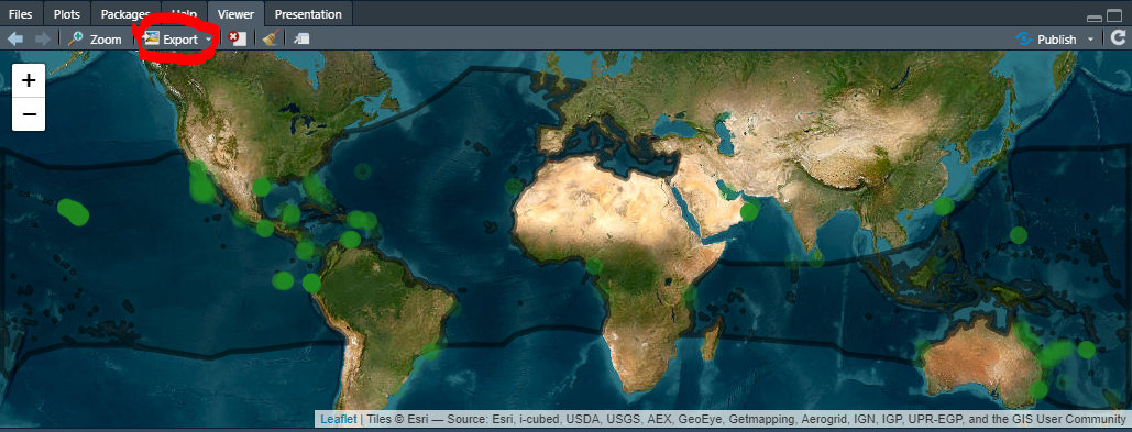
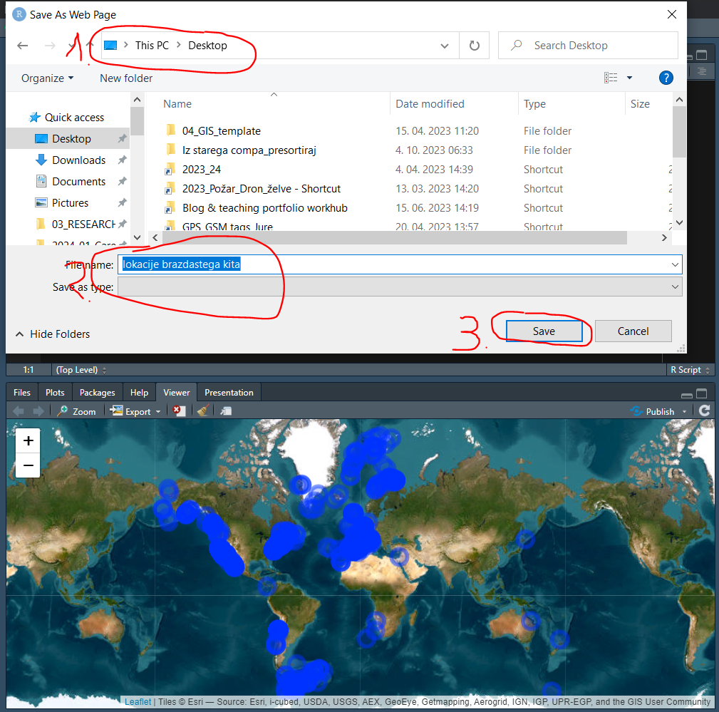
We can export the map in the html format, which will retain its interactive properties:

Click Export button in the viewer

Select Save as web page

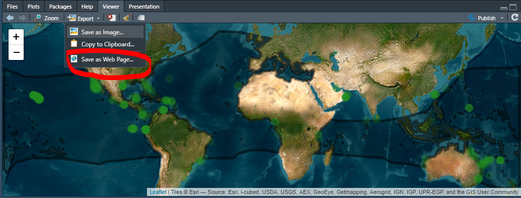
Set the file name, choose location on our computer (Desktop) and click Save

Questions to consider:

What is GBIF and how can it be useful for your research/teaching?
What are the drawbacks of the GBIF data considering that some of it comes from citizen science?
How many times do you need to run install.packages() functions and how many times the library() function?
Which package and functions are easy to use for filtering and selecting only the data of interest?
Which package and functions are easy to use for simple spatial data visualization of spatial points?

Do you have any questions?

Task

Today your task will be more challenging than those of yesterday. Follow the next steps to accomplish it:

Choose one marine species (your favorite) and find its Latin name.
Open new R script, save it to desktop and name it Accessing "insert your species name" data with R on the desktop.
Copy - paste all R code that we ran for fin whale example (you can exclude only install.packages(), as the packages are already on your computer now).
Adapt the code in a way that you replace Balaenoptera physalus with chosen species name and rename physalus_gbif according to your species (i.e. Liza aurata & aurata_gbif).
Add the argument limit = to occ_search() function and download more than 500 occurrences (change 500 with a number of your choice).
Extract the data part of the *_gbif object and rename the object according to you species (i.e. aurata_data).
1. if there are zero or a small number of occurrences of your species (< 100), repeat from step 1.
2. if there are > 100 occurrences of your species, proceed to step 7.
Select only meaningful columns from the *_data dataframe. The column names should be the same as in the fin whale example and the code should work on your data. Add a minimum three columns to the select function on top of the ones that I chose to select!
Apply filter to your data and try to change the filtering value of coordinate uncertainty to correspond to your species better (i.e. 500 metres might be better for Liza aurata).
Display the filtered occurrences of your species on a leflet map. Explore the available base maps here and change it to one of your choice (i.e.replace "Esri.WorldImagery" with "Esri.WorldImagery" or "OpenTopoMap".

If something doesn’t work straight away, first think about the problem/error, consult a neighbor on your left, then on your right. If after that you still don’t know how to fix the problem or proceed, ask me for help!

Task

Save both R scripts, so you can reuse your code in the following labs.

When you close R studio, select Yes when it asks if you want to save your work-space.

Partly funded by EU Erasmus+ Programme for Higher Education Staff Mobility